Entropy coding by a beginner for beginners - Part 1: Code Length

Introduction

Once upon a time, when I had just got introduced to C, one of the initial projects that I chose to make was a steganography program. The idea didn’t seem too difficult. At that time, I was barely able to assemble lines of code together and just didn’t think of searching for libraries to encode and decode .png and .jpeg files (I wasn’t even aware of the existence of stb libraries back then). However, thanks to that, I got introduced to compression right from the start. I tried something, didn’t quit grasp fully what I did, and moved on to something else. Years later, I decided to revisit this topic because the concept of “compressing” information intrigued me since that time. But this time, I decided to document it because, as it is said:

“The best way to learn is to teach.” — Frank Oppenheimer

This series of articles is for those who are just beginning to explore the world of compression. So, if you already have experience or make compression for living you won’t find any new information here. But in this case, if you come across any glaring errors, I would appreciate it if you could reach me out so that I can correct them.

Now let’s begin.

Kraft-McMillan equation

When we use Huffman for entropy encoding, in general, we can only represent probabilities that are equal to two to the negative power of two. What does it mean, and is it bad? Let’s briefly examine these questions.

At start let’s look at the Kraft–McMillan inequality. It works for any B-ary system, but all the rest of the formulas will assume a binary system automatically.

\[\sum_{x \in S} \frac{1}{2^{l(x)}} \le 1\]

Here, S is a set of our symbols or simply an alphabet, x is a symbol in this alphabet, and l is the length of code for a particular symbol. That is, $S = \{x_0, x_1, x_2, \dots\}$ and $|C(x)| = l(x)$. Accomplishing these conditions gives us the guarantee that we have codes for our symbols that we can later decode unambiguously. From this inequality, we can find a formula for $l(x)$ of the symbol.

\[p_i = \frac{1}{2^{l_i}}; \; 2^{l_i} = \frac{1}{p_i}; \; l_i = log_2 \frac{1}{p_i} \; or \; l_i = -log_2 \ p_i\]

You can think of p as the probability that it generally is. Let’s consider an example where we have Huffman codes for some symbols.

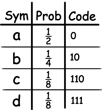
Checking it:

\[\frac{1}{2^{-1}}+\frac{1}{2^{-2}}+\frac{1}{2^{-3}}+\frac{1}{2^{-3}} = 1\]

The condition is accomplished, and we really can unambiguously decode a sequence of such codes. For example, 01101110 = acda. Currently, the average code length for our alphabet from above, with such a probability distribution is $L = 1.75$ bits. We can calculate this using the formula below:

\[L = \sum_{x \in S} \ p(x) * l(x)\]

If we try to reduce average code length by reducing the code for the symbol ‘b’ to just 1 instead of 10 (because the probability for ‘b’ is higher than ‘c’ and it seems logical to choose ‘b’ because of this), then we will have:

\[\frac{1}{2^{-1}}+\frac{1}{2^{-1}}+\frac{1}{2^{-3}}+\frac{1}{2^{-3}} = 1.25\]

We ran out of our budget, and according to the inequality, we should not be able to unambiguously decode our code sequence. Let’s check: 01101110 = abba.. or ac..? Who knows? As we can see, the inequality didn’t lie to us. In fact, we can’t get shorter codes for such probability distribution. That is, they are optimal for the given probability distribution. In order to understand why, we first need to define a measure of information that we process or better to say, a measure of unpredictability/”possible choice” of the information we process. Entropy is what we need for such measurement.

Shannon entropy

The concept of entropy is kind of broad on its own. We are interested specifically in Shannon entropy (H) from information theory, and the formula for it looks like this:

\[H = -\sum_{} p_i * log \ p_i\]

As the author noted himself in his work, the formula that he came up with to satisfy the requirements he set for the measure of “information” from some “source of information” was very similar to the definition of Boltzmann-Gibbs entropy from statistical thermodynamics (just a fun fact). If you ask me to try to give intuition behind the calculation of H, then I would highlight the following two properties. First, why logarithm? The value of a logarithm will grow linearly with the increase of possible options by the base of this logarithm. The base of the logarithm is chosen based on the unit of measurement. Since we are working with binary, our logarithmic base will be 2. For example, $log_2 \ 128 = 7$ and $log_2 \ 256 = 8$ but $log_2 \ 384 = 8.58$. Thus, we can write down the formula like this:

\[H_2 = -\sum_{} p_i * log_2 \ p_i\]

In general case when we are talking about entropy in computer science (and especially in information theory), we assume a base of 2. So we can just write $H$ instead of $H_2$. Usually, this is clear from context. From now on, I also will write just $H$. Second, why is it necessary to multiply the result of the logarithm by the probability? By doing this, we weight the result of our logarithm. In this way if we would have $n$ symbols and all of them have the same probability $(1/n)$, then our $H$ will be equal to $log_2 \ n$. For example, if we have 256 symbols and the probability of each one is $1/256$, then $H = 8$ instead of 2048.

If you notice, the calculation of average code length for Huffman codes is kind of similar to the entropy formula. This is because the former is an approximation to the latter and differs in that for entropy we use $-log_2\ p$. In principle, this seems logical, since for an event with a probability of 50% or 0.5, we need 1 bit, that is, codes will be 0 and 1. But for an event with a probability of 0.9, by this logic, we would need roughly only 0.15 bit. Thus, sometimes you can hear that compression is close to the entropy or Shannon limit. At that time, data compression was literally just being born, and Huffman codes were a good approximation of entropy for textual data. We can check how much Huffman codes deviate from entropy in the following way:

\[D = (L - H) / H\]

For the source of information from pic.1, D = 0. Let’s look at the next example with a more skewed probability distribution:

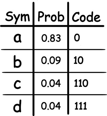
In this case, L = 1.25, H = 0.9, and D = 0.39 or 39%.

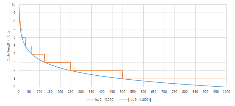
The graphic above only shows the correspondence between a code length and a given probability, and it does not tell the whole story. By using Huffman for encoding, we “round up” our probability toward the closest free slot of probability of $2^{-n}$. That it, the larger our alphabet is, and/or the closer probability of each symbol will be to $2^{-n}$, the more optimal Huffman codes will be for this case (you can check this post of Yan Collet, author of zstd, for some additional info about this).

Let’s look at the last two examples for an alphabet of 5 symbols. In the first case, let all symbols have a probability of 0.2. The resulting Huffman codes would look like this (00, 10, 11, 010, 011). L = 2.4, H ≈ 2.32 and have D ≈ 3.45%. In the second case, let’s take a probability distribution like (0.96, 0.01, 0.01, 0.01, 0.01). Then we will get codes like (0, 100, 101, 110, 111). We have L ≈ 1.08, H ≈ 0.32 D = 237.5%. In this case, we lose a solid amount of bits by giving a probability of 0.96 a whole bit.

Final words

By using Huffman, we can encode our probability only using a discrete amount of bits. But at the same time, decoding Huffman codes by using table method requires a very small amount of operation for decoding symbols. In addition, if count a possibility for compact representation of Huffman table, this method should not be neglected. It just serves as a possible alternative that you can choose from. We only looked at static probabilities for symbols because attempting to make Huffman adaptive, that is, taking into account the statistics of the appearance of each symbol at the time of encoding process, would require rebuilding the codes tree and, as a consequence, would not allow us to use the table method for decoding. That, in turn, means that we lose the main advantage of Huffman. For making our encoder adaptive, we have better options, and we will explore them in the next parts.