Entropy coding by a beginner for beginners - Part 2: Arithmetic Coding

Introduction

The group of methods for encoding еntropy that can do this with a fractional part of code length is called arithmetic coding (AC for short). In this part, we will look at how the classical version of AC works. If you are planning to use one of the AC methods in your project, it’s better to check if it is under patent or something.

If you have decided to really delve into compression, then facing with AC is inevitable. When you hear for the first time that there is exist a possibility to encode something using fractional bit lengths, it feels like something crazy. My introduction to AC was completely wrong and confusing because I started from scratch and didn’t understand what I was trying to figure out at all. I also started with a fairly new AC method, which was also very wrong without knowing the basics. It’s just that at that time I thought it was the same, conceptually this may be true, but they have different implementations and properties. That’s why I know for myself that if you start learning how AC works, knowing only its “name”, it can be quite frustrating. At the end I listed materials that if I had found at the start would have saved me a lot of time in understanding AC. I’ll try to give just another form of explanation with code examples, which I hope will help to build the picture of how it works faster.

The main idea of AC encoders is to try to increase (or decrease) the base by the amount of entropy needed to encode a symbol with some probability, in such a way that it will then be possible to unambiguously decode this increase (depending on the encoder, it can be both FIFO or LIFO). When I said to increase by entropy, I meant the following operation: our base is 16384 which is $log_2 = 14$ bits. We have to encode a symbol with a probability of 0.9 that requires 0.15 bits. Now our base will be equal to 14.15 bits of entropy. That means if we repeat this operation 5 times, our base will be 15 bits. We encoded 6 values, but our base has grown only by 1 bit. This is just an illustration of what I mean, so don’t focus on it, but in this way, with a pinch of math, this is what happens. How exactly the base is represented and the increase happens depends on the AC realization. Very soon we will see how we can do this, but first, we can make some conclusion. Our base should be big enough to have the capability to encode values in itself. For example, $log_2 \ 4$ - $log_2 \ 2$ will be 1 bit, but it’s obvious that this is not the same as $log_2 \ 32768$ - $log_2 \ 16384$ where the difference is also 1 bit. In the first case, we just don’t have enough resolution to encode something in between.

Big picture

When we use the classic AC to encode our probability, we build one long floating point number that in between 0 and 1, which we can decode in FIFO order. The first thing to know is that now we don’t encode probability as a single number but as a range of CDF (Cumulative distribution function).

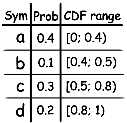
This is necessary so that we can distinguish between the symbols that we are encoding. The general idea of how AC works is shown below.

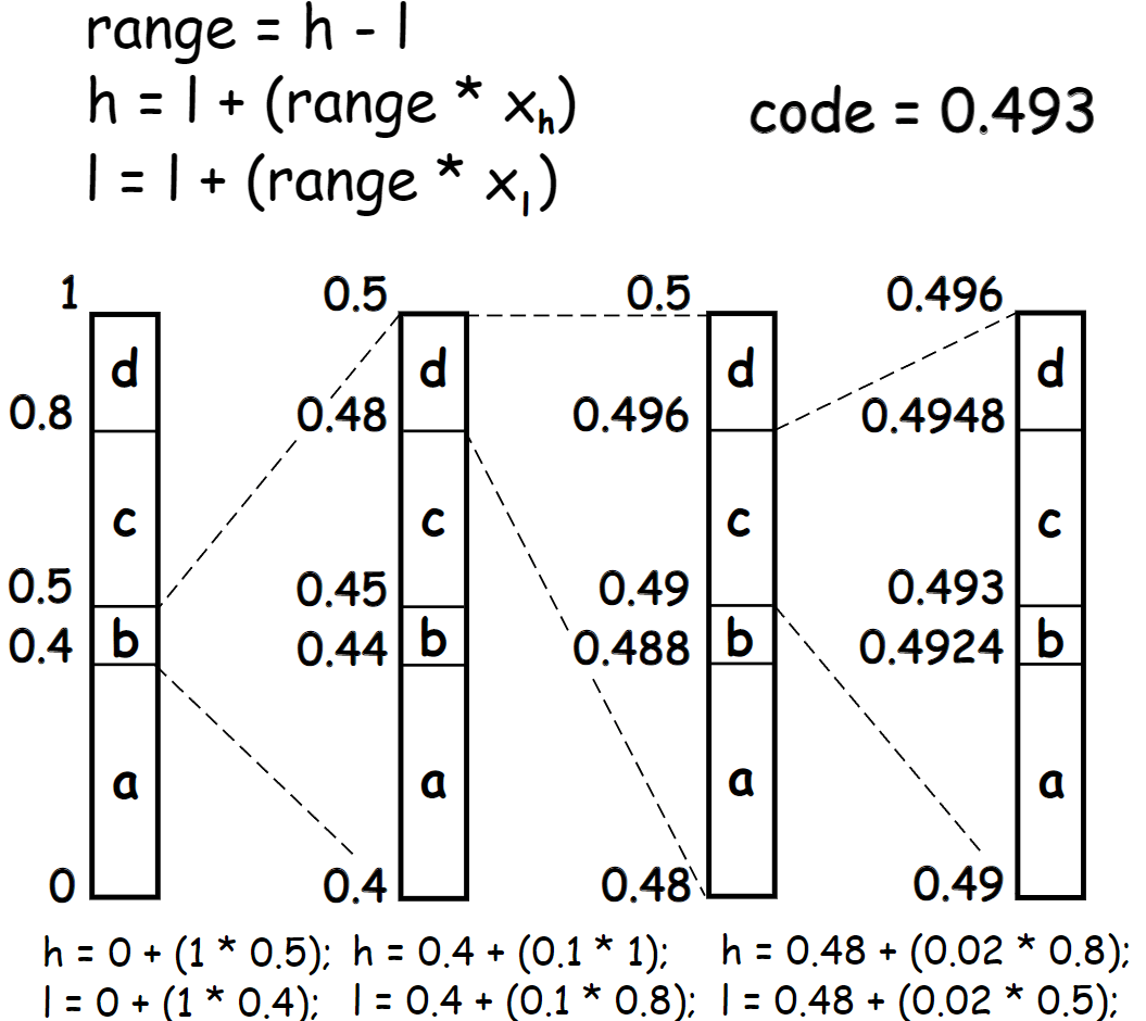
The decoding process is nearly identical in this simplified scheme. First, we try to find a range to which the code belongs, and then update our interval by the range of the decoded symbol.

0.4 >= 0.493 < 0.5 (b)
0.48 >= 0.493 < 0.5 (d)
0.49 >= 0.493 < 0.496 (c)

We are basically building an infinitely small number by adding information to it from the significant part (MSB). It’s the adding of information from the MSB that allows us to decode our symbols in FIFO order. If you don’t see why and why we must track both high and low and not only one of them, then this will become clearer when we start implementing it.

Encoding

Finite precision

We have just seen an example of how it would work if we would had infinite precision. In order to implement the algorithm in practice, we must decide how we will store our high and low values and CDF range for symbols. Using float point will be impractical since this format can only store a limited number of symbols encoded in this way and the accuracy is limited. If you are not familiar with floating point format, you can try to play with it here. So, I’ll go straight to fixed point format. I would like to point out in advance that all rules for encoding and decoding work kind of “together”, so for you, as for me, it may not be obvious why some operations make sense. In this case, just keep reading, maybe it will become clear later.

First, let’s decide on high and low storage format. As you can see from the example of the algorithm execution, these are the values that we use to store information about all encoded symbols. We can say that they are our base. From the first picture (and the previous part), we can conclude that the high of our range should never be equal to one. This means that our range for low and high is [0, 1), and the same will applie for CDF. An open interval means that our number can be infinitely close to one but never be equal to it e.g., 0.99(9).

high = 0xFFFFFF(F…)
low = 0x000000(0…)

We operate with low and high value in the register, and of course it can’t fit infinite values inside (no thanks, please). But we assume that beyond the LSB boundary, we have an infinite number of 1’s for high and 0’s for low. A bit later I will show how we are gonna use this. The representation of CDF is kind of similar in the way that we have values that are between 0 and 0.99(9), but we save it as an integer number and count it relative to the total sum of CDF. We can calculate what range some symbol takes, like:

X_h = CDF[S_h] / CDF[Total]
X_l = CDF[S_l] / CDF[Total]

Next questions are how many bits of our base we should have and what maximum value should be allowed for our CDF to store? Let’s first look at how we operate with our low, high and CDF values at all. The formula from the second picture only works if our numbers are between zero and one. We also can’t use the formula for CDF range above since we work with integers and such division will always give us 0. Hence our formula will look like this:

high = low + ((range * CDF[X_h]) / CDF[Total])
low = low + ((range * CDF[X_l]) / CDF[Total])

We will work with a 32 bits register. This means that in order to avoid overflow during multiplication range * CDF[X], the maximum values of these numbers must satisfy the following requirement.

MAX_USED_BITS >= CODE_BITS + FREQ_BITS

Here, CODE_BITS is the value for low and high, and FREQ_BITS is for CDF. Additionally, we also have the following limitation:

CODE_BITS >= FREQ_BITS + 2

That is, by using 32 bits, we can choose our values as 17 and 15 bits. But, to make initialization easier, I have chosen 16 and 14 bits (this will not significantly affect the final compression result). In order to explain why we have the second constraint, we must first consider the decoding part. We will get to it soon and return to this question, but for now, we can write it down as:

//ac_params.h
static constexpr u32 CODE_BITS = 16;
static constexpr u32 FREQ_BITS = 14;
static constexpr u32 FREQ_VALUE_BITS = 14;
static constexpr u32 PROB_MAX_VALUE = (1 << FREQ_BITS);
static constexpr u32 CODE_MAX_VALUE = (1 << CODE_BITS) - 1;
static constexpr u32 FREQ_MAX_VALUE = (1 << FREQ_VALUE_BITS);

struct prob
{
   u32 lo;
   u32 hi;
   u32 scale;
};

Data for our AC coder

class ArithEncoder
{
    u32 lo;
    u32 hi;
}

And finally beginning of encoding function.

//ac.cpp
void ArithEncoder::encode(prob Prob)
{
    u32 range = (hi - lo) + 1;
    hi = lo + ((range * Prob.hi) / Prob.scale) - 1;
    lo = lo + ((range * Prob.lo) / Prob.scale);
    ...
}

The calculation of the new ranges looks almost the same as in the formula above. Adding and subtracting one is necessary because we have an open interval in our high variable. As was said before, beyond LSB boundary, we have an infinite number of 1’s. Since we are infinitely close to the next number, not adding one will count as rounding (at least in this implementation of AC). We subtract it for the same reason. If we ignore this operation, it will bring us to a situation when we are not being able to decode our data right.

Normalization

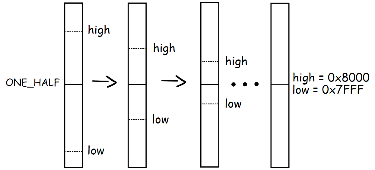
The next step is normalization. As soon as we change our low high range, all subsequent ranges will stay inside the previous one. This means that if our first range becomes e.g. 0.1– 0.4, then values beyond this range will never be used. In the context of a fixed point, this means that these are bits that will never change in subsequent calls, so we can write them down. If the value of hi less than 0.5, then it will never get greater than that and we can write 0 to the output stream. If the value of lo gets greater than 0.5 for same reason write 1.

After that, we can shift out the MSB that we have already written and that will never change, and in place of the new LSB put bit from the infinite pool. Basically, we are doing rescaling for our range.

//ac.cpp
void ArithEncoder::encode(prob Prob)
{
    ...
    for (;;)
    {
        if (hi < ONE_HALF)
        {
            writeBit(0);
        }
        else if (lo >= ONE_HALF)
        {
            writeBit(1);
        }
        else break;
      
        hi <<= 1;
        hi++;
        lo <<= 1;
        hi &= CODE_MAX_VALUE;
        lo &= CODE_MAX_VALUE;
    }
}

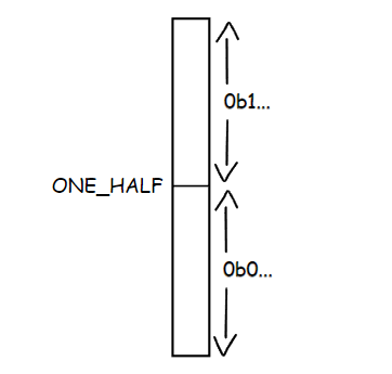
It’s not always that simple; occasionally, we can have situation like this:

That is, neither high nor low will go beyond ONE_HALF, which means that their MSB are different, but the interval between them is getting smaller and smaller. After some period, it will be impossible to encode a value in between. We will track additional two boundaries for high and low value to solve the problem of knowing when they are on their way to convergence.

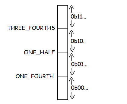
//ac_params.h
static constexpr u32 ONE_FOURTH = (1 << (CODE_BITS - 2));
static constexpr u32 TREE_FOURTHS = ONE_FOURTH * 3;
static constexpr u32 ONE_HALF = ONE_FOURTH * 2;

Let’s complete our encoding function like this and then discuss what’s going on here.

//ac.cpp

class ArithEncoder
{
    ...
    u32 PendingBits;
}

void ArithEncoder::encode(prob Prob)
{
    ...
    for (;;)
    {
        if (hi < ONE_HALF)
        {
            writeBit(0);
        }
        else if (lo >= ONE_HALF)
        {
            writeBit(1);
        }
        else if ((lo >= ONE_FOURTH) && (hi < TREE_FOURTHS))
        {
            ++PendingBits;
            lo -= ONE_FOURTH;
            hi -= ONE_FOURTH;
        }
        else break;
        ...
    }
}

void ArithEncoder::writeBit(u32 Bit)
{
    fillBitBuff(Bit);

    u32 ReverseBit = !Bit & 1;
    while (PendingBits)
    {
        fillBitBuff(ReverseBit);
        --PendingBits;
    }
}

In the third case, we write nothing to the output stream. Instead, only make a note about that there was a rescaling to PendingBits and wait for an opportunity to write these bits. This part is probably the hardest to understand, and until I saw a visual explanation of this step[4], I couldn’t fully understand why it working. The fact is that we, in any case, need to avoid convergence. We cannot leave our ranges as they are. We don’t know yet, at the current scale, which MSB will not change in the future, but later, on a more global scale, we get this information.

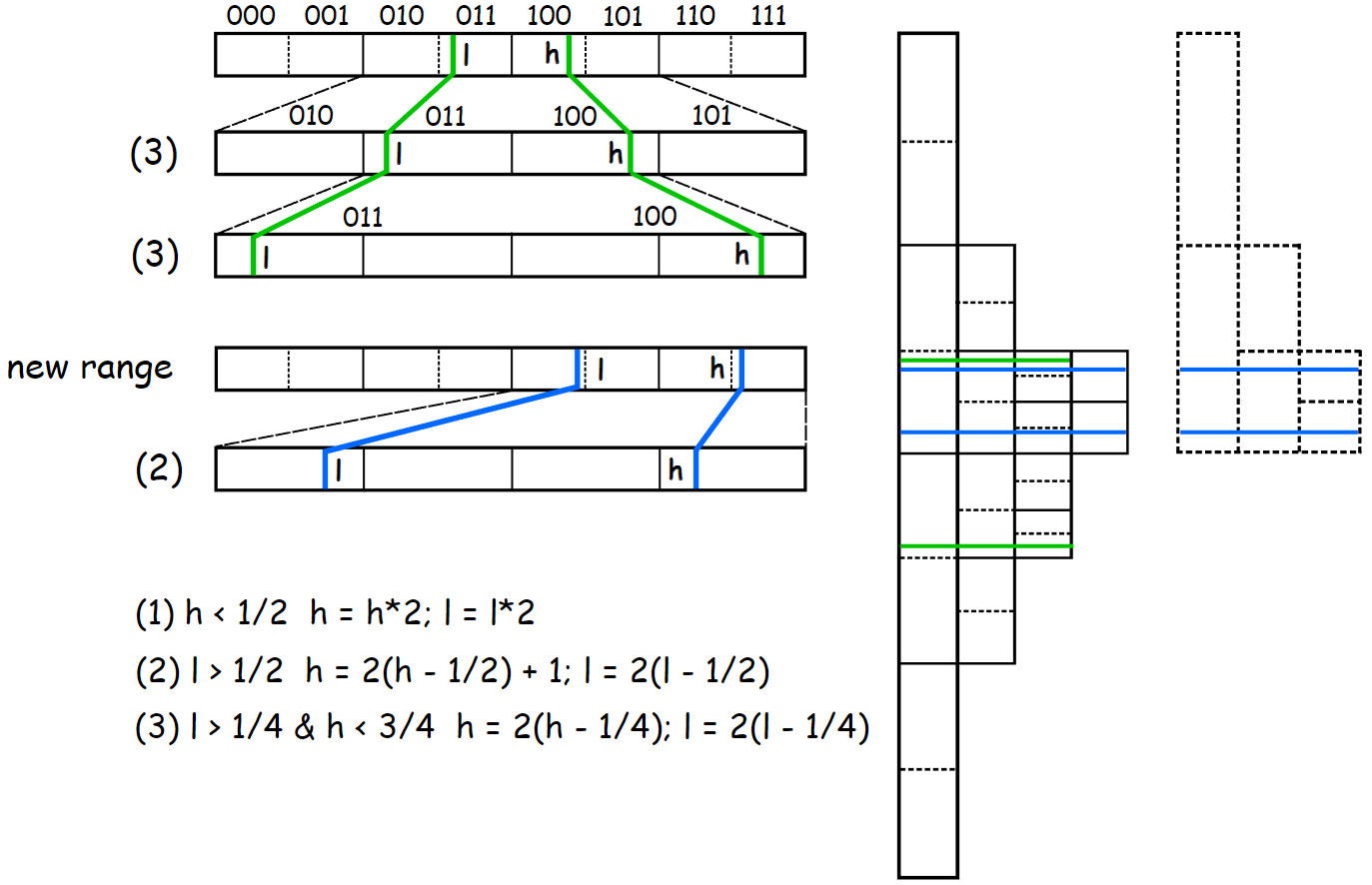
As you can see, such a transformation lead to same result.

End of stream

The last thing we need to do is have the ability to unambiguously decode our last encoded symbol. In my first example, I just take the average between 0.49 and 0.496. In practice, we do something similar. We only need to add a few bits to our sequence to uniquely decode the last character.

void ArithEncoder::flush()
{
    PendingBits++;
    if (lo < ONE_FOURTH) writeBit(0);
    else writeBit(1);

    if (BitBuff) Bytes.push_back(BitBuff);
}

This is how encoding happens. The larger the CDF range a symbol occupies (that is, the higher its probability), the less we narrow our low and high range, which is why compression occurs.

Decoding

Now let’s take a look at the decoding part.

class ArithDecoder
{
    u32 lo;
    u32 hi;
    u32 code;
    ByteVec& BytesIn;
}

Instead of PendingBits, we have code where we store bits that we took from the encoded stream. So, first, we initialize our code variable to start the decoding process like this.

ArithDecoder(ByteVec& InputBuffer): BytesIn(InputBuffer)
{
    for (u32 i = 0; i < 2; ++i)
    {
        code = (code << 8) | getByte();
    }
}

Since CODE_BITS is 16 bits, we just need two bytes. The next step is to get the value that was encoded. In the example from the second picture, we are simply comparing with the current range in the high and low scale, but we can also get an approximate value of the encoded CDF symbol by doing the following operation.

range = high – low
value = (code – low) * range

For the first step from pic.1, this operation will return 0.493, but on the second step, we will obtain 0.93, which falls within the CDF range for the symbol ‘d’. This is how we will obtain our encoded symbol values at each step. We consider only a fraction of the encoded number and cannot compare it directly as shown in the image. Actually, it’s not exactly true. For binary AC it is no need to do this reverse transformation. It’s just for a non-binary alphabet this method is more optimal than converting each CDF range to the current range of high and low and comparing them on that scale. So, our function for obtaining the current encoded frequency looks like this:

u32 ArithDecoder::getCurrFreq(u32 Scale)
{
    u32 range = (hi - lo) + 1;
    u32 ScaledValue = ((code - lo + 1) * Scale - 1) / range;
    return ScaledValue;
}

CDF constrain

During encoding, we first multiply by range and then divide by Scale. Now we perform the reverse operation. At this step, we can go back to our question of why this constraint CODE_BITS >= FREQ_BITS + 2 is needed. It’s all because we divide by the range. When we do this, we expect to get the smallest value that the CDF has. We can’t exclude the possibility that this might be the case for some symbols.

CDF[high] - CDF[low] = 1

If the range on which we divide is even less by one than the range of our CDF, at one point we won’t be able to decode such a symbol because we will be in a wrong CDF range and our compression will simply be useless. The lowest range that can be between high and low we can find out by looking at normalization scheme, and this will be when high == TREE_FOURTHS and low == ONE_HALF – 1, or high == ONE_HALF and low == ONE_FOURTH - 1. That’s why we need that our high and low values must be at least 4 times greater than max CDF value.

Normalization

Updating the range looks nearly the same, only that now we have the code for which we must do the same operation as for high and low, since normalization now signals to us when we should grab new bits from the encoded stream.

void ArithDecoder::updateDecodeRange(prob Prob)
{
    u32 range = (hi - lo) + 1;

    hi = lo + ((range * Prob.hi) / Prob.scale) - 1;
    lo = lo + ((range * Prob.lo) / Prob.scale);

    for (;;)
    {
        if (hi < ONE_HALF)
        {
        }
        else if (lo >= ONE_HALF)
        {
        }
        else if ((lo >= ONE_FOURTH) && (hi < TREE_FOURTHS))
        {
            code -= ONE_FOURTH;
            hi -= ONE_FOURTH;
            lo -= ONE_FOURTH;
        }
        else break;

        hi <<= 1;
        hi++;
        lo <<= 1;
        hi &= CODE_MAX_VALUE;
        lo &= CODE_MAX_VALUE;

        code = shiftBitToCode();
        code &= CODE_MAX_VALUE;
    }
}

Comparison with Huffman

That’s what AC looks like. The main advantage of this method of encoding entropy is that we don’t have a hard restriction on the source from which we take our probability to encode, namely the CDF value. Only that CDF[Total] must not exceed FREQ_BITS. This allows us to change the probabilities during the encoding/decoding process, which means that we can make our probability estimates adaptive.

The encoder by itself only encodes the ranges and their interpretations is our business.

Below is a comparison of compression (if we take the count of occurrence of each individual byte from the entire file) between a simple Huffman implementation with a maximum code length of 12 bits and the above AC with a maximum CDF value of 2^14 which was optimally normalized. We haven’t looked at how we encode values with AC and how to do normalization for CDF yet, so for now, it’s enough to understand that if we try to map a frequency counts for bytes whose total sum is greater than maximum value that can hold a chosen CDF range, there will be variation in who should take shorter codes and who should take longer codes. The optimal method will give CDF values that result in the smallest compression. Decoding was done without auxiliary data struct. Also, if we know that CDF[Total] == 2^n we can replace some divisions with shifts. I didn’t do that for the test. (c/s means clock/symbol).

Result for AC

name	H	file size	compr. size	bpb	enc c/s	dec c/s
book1	4.572	768771	435102	4.528	228.4 (16.2 MiB/s)	318.8 (11.6 MiB/s)
geo	5.646	102400	72278	5.647	271.4 (13.7 MiB/s)	318.2 (11.7 MiB/s)
obj2	6.26	246814	193160	6.26	297.3 (12.5 MiB/s)	339.6 (10.9 MiB/s)
pic	1.21	513216	77951	1.215	81.3 (45.7 MiB/s)	110.2 (33.7 MiB/s)

Result for Huffman

name	H	file size	compr. size	bpb	enc c/s	dec c/s
book1	4.572	768771	439247	4.57	13.4 (277.9 MiB/s)	13.6 (273.9 MiB/s)
geo	5.646	102400	72840	5.69	11.3 (328.4 MiB/s)	12 (308.1 MiB/s)
obj2	6.26	246814	194582	6.3	14.3 (260.3 MiB/s)	14.6 (253.9 MiB/s)
pic	1.21	513216	107443	1.675	9.1 (407.5 MiB/s)	9.4 (396.3 MiB/s)

For most files, the difference is not that big, if we simply take the frequency of bytes from whole files and use it to make compression, but I think the first thing that catches your eye is the difference in c/s between these two methods. It’s also quite interesting how the pic that has less entropy and therefore spends less time looping around in the normalization loop has fewer c/s. That is, it turns out that the cost of encoding/decoding can be pretty uneven for different types of data.

Rearranging division

We can do a small rearrangement of math to reduce the amount of division operation for encoding to one (and if we change the API for decoding also, but I haven’t done this), rewriting range scaling in this way:

void encode(prob Prob)
{
    u32 step = ((hi - lo) + 1) / Prob.scale;
    hi = lo + (step * Prob.hi) - 1;
    lo = lo + (step * Prob.lo);
    ...
}

To make this work, we also need to change values for CODE_BITS і FREQ_BITS. The thing is, by rearranging the divide operation, we’re reducing our encoding precision. It now becomes CODE_BITS - FREQ_BITS, whereas in the previous case, it was always from 16 to 15 bits. Due to the fact that there is now no overflow occuring on multiplication, the maximum value of CODE_BITS can now take 31 bits, but I set it to 24 bits for ease of initialization and simply because we are not taking advantage of 31 bits in this implementation.

name	H	file size	compr. size	bpb	enc c/s	dec c/s
book1	4.572	768771	435236	4.528	228,1 (16.3 MiB/s)	262,4 (14.1 MiB/s)
geo	5.646	102400	72296	5.647	280,8 (13.2 MiB/s)	254.2 (14.6 MiB/s)
obj2	6.26	246814	193202	6.26	283,1 (13.1 MiB/s)	278.2 (13.3 MiB/s)
pic	1.21	513216	78031	1.215	84,4 (44 MiB/s)	102,5 (36.2 MiB/s)

Despite the decrease in accuracy, the result did not get much worse. The reduction of division operations did not produce a “wow effect” in terms of encoding speed. The benchmark result was at a level of error, so I don’t want to fool you and choose the best one. Interestingly, although the number of divisions for decoding remained the same, it seems that the dependency graph of instructions is better handled by my CPU in this way (actually the result varies between compilers). Several MiB/s is of course cool, but it certainly would be better if it ware more. It’s not surprising that the encoding process is so tight. It might be fine if we do some simple loop during normalization, but only branch misses are nearly 30% and greater (depending on data entropy). The ability to set CODE_BITS to 31 bits, which will allow us to normalize a byte at a time instead of bit by bit, is essentially the main advantage of changing the division order. Shifting a whole byte at a time with 16 bits CODE_BITS means that we will be waiting until the 8 MSB bits become identical, and as a result, the precision of the range would shrink to 8 bits, which in turn adds constraints to the max value for CDF. But what is more important is that such normalization scheme will not work for a byte at a time. The canonical implementation for multi character (since binary came before) AC with byte at a time normalization is probably Michael Schindler version. You can read about how and why it works starting from this post by Charles Bloom. You just won’t find anywhere else to read about it, at least I didn’t. If you’re new to compression and haven’t come across Charles’s blog, it’s one of the main source of information about compression on the internet at all, by the way.

In the next parts, I will be using the version of AC that I showed, so keep that in mind. If I show some benchmark then it is very likely that later I will add the result for the bytewise normalization version of AC below. If my explanation will be useful for people who are just getting into compression, then I’ll try to make a post like this for AC with bytewise normalization.

Source code for this part.

References

[1] Arithmetic coding for data compression https://web.stanford.edu/class/ee398a/handouts/papers/WittenACM87ArithmCoding.pdf

[2] Data Compression With Arithmetic Coding https://marknelson.us/posts/2014/10/19/data-compression-with-arithmetic-coding.html

[3] Arithmetic Coding + Statistical Modeling = Data Compression https://marknelson.us/posts/1991/02/01/arithmetic-coding-statistical-modeling-data-compression.html

[4] Rescaling operations for arithmetic coding https://www.youtube.com/watch?v=t8_198HHSfI&list=PLE125425EC837021F&index=45

[5] Rant on New Arithmetic Coders http://cbloomrants.blogspot.com/2008/10/10-05-08-5.html